Sharding Large Models with Tensor Parallelism
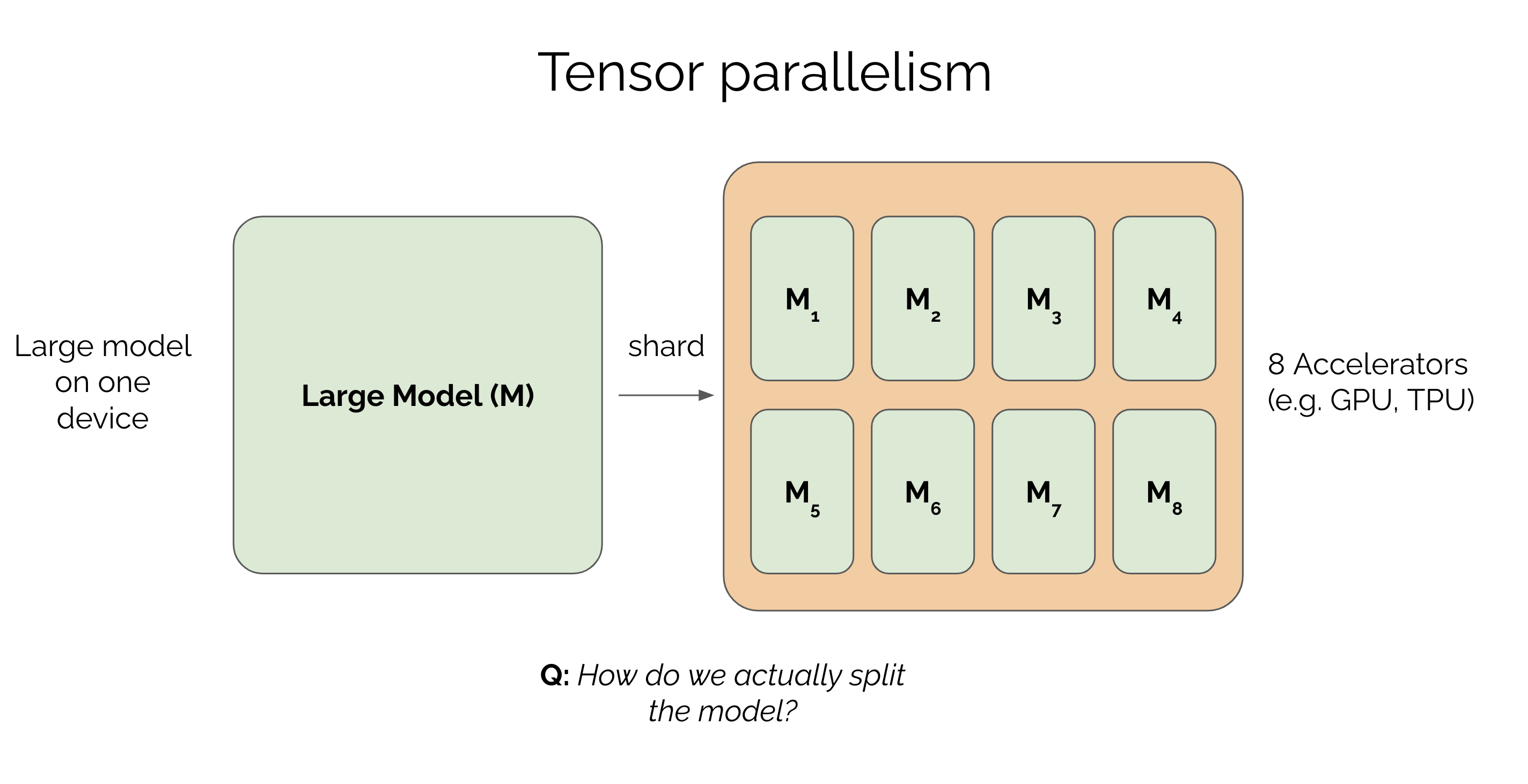
In a previous post, we covered how to parallelize the data in a large model across multiple GPUs. We saw that if you can't fit an entire batch on a single GPU, you can split the batch across multiple devices. But what happens when the model is so big that even with a batch of 1 you can't fit it on a single GPU? Or the model fits but trains too slowly? We can accelerate training by parallelizing the model itself. This technique is called model parallelism. In this post, we'll mainly cover a type of model parallelism called tensor parallelism which is commonly used to train large models today.
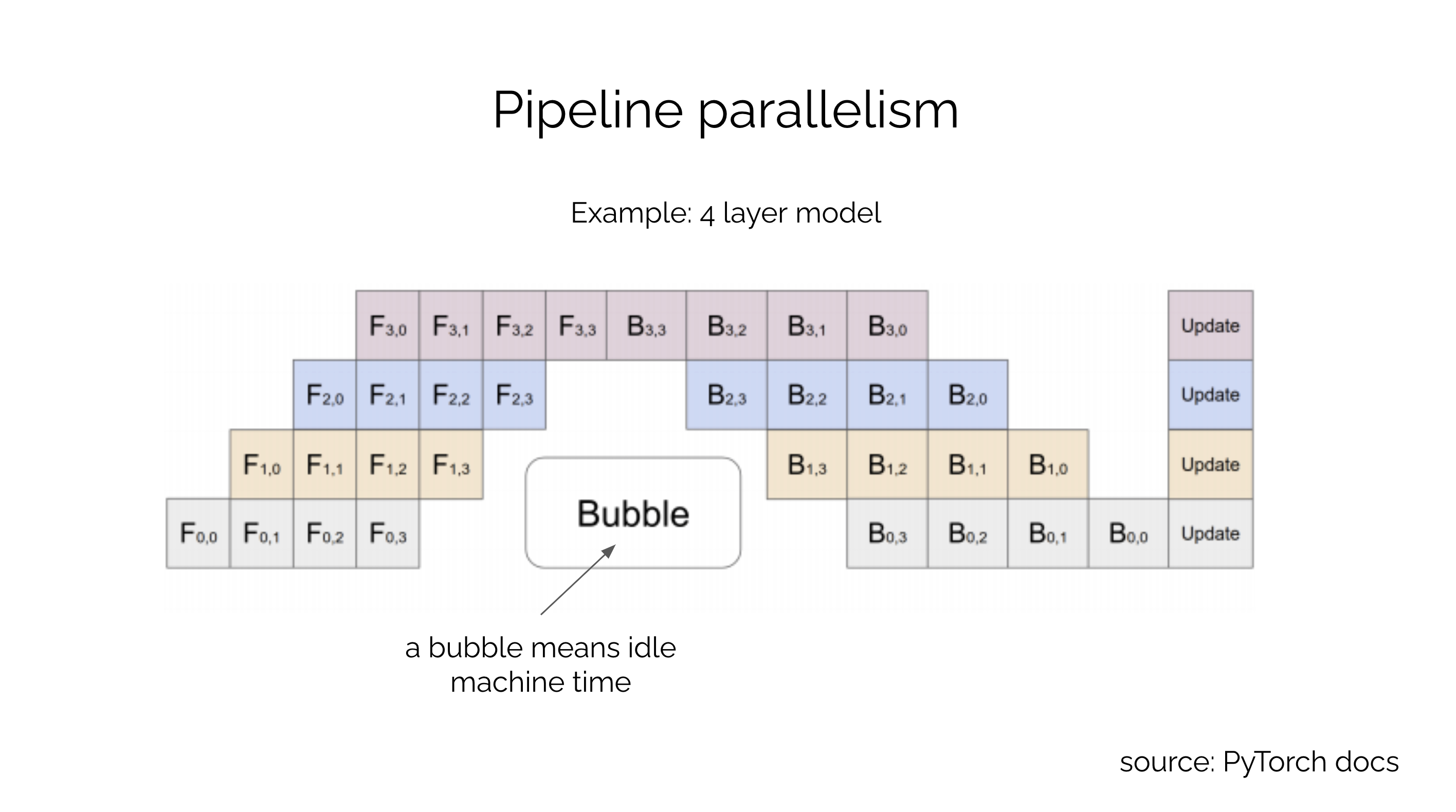
Pipeline parallelism and its limitations
There are many ways to parallelize a model. One of the most intuitive approaches is called pipelined model parallelism. In this approach, the model is split into multiple stages, and each stage is assigned to a different device. The output of one stage is fed as input to the next stage. For example, if you're pipeline parallelizing an 8 layer MLP across 8 devices, you would place a layer on each device. The output of the first layer would be fed as input to the second layer, and so on. The output of the last layer would be the output of the MLP (see the PipeDream (opens in a new tab) paper for details). While simple, this approach is not very efficient and suffers from idle time when machines are waiting for other machines to finish their stages. This is because the pipeline is waiting for a stage to finish in both the forward and backward pass. Machine idling, referred to as a bubble, is inefficient because the machine is not being utilized during a bubble.
Efficient model sharding with tensor parallelism
How can we parallelize a model more efficiently? Rather than parallelizing the model layer by layer, we can split the model into shards that are distributed across multiple devices and execute in parallel. This approach is called tensor parallelism or model sharding. It is usually more efficient than pipelining but can be more challenging to implement, because it requires careful consideration of how to split different parts of the model. In this post, we'll cover how to parallelize an MLP using tensor parallelism with an approach popularized by the Megatron paper (opens in a new tab).
Let's consider a 2 layer MLP with layer 1 parameterized by matrix A and layer 2 parameterized by matrix B. Now let's say we have a batch of data and we want to compute the output . In a typical MLP, we would compute and where is the activation function. So how can we parallelize this model?
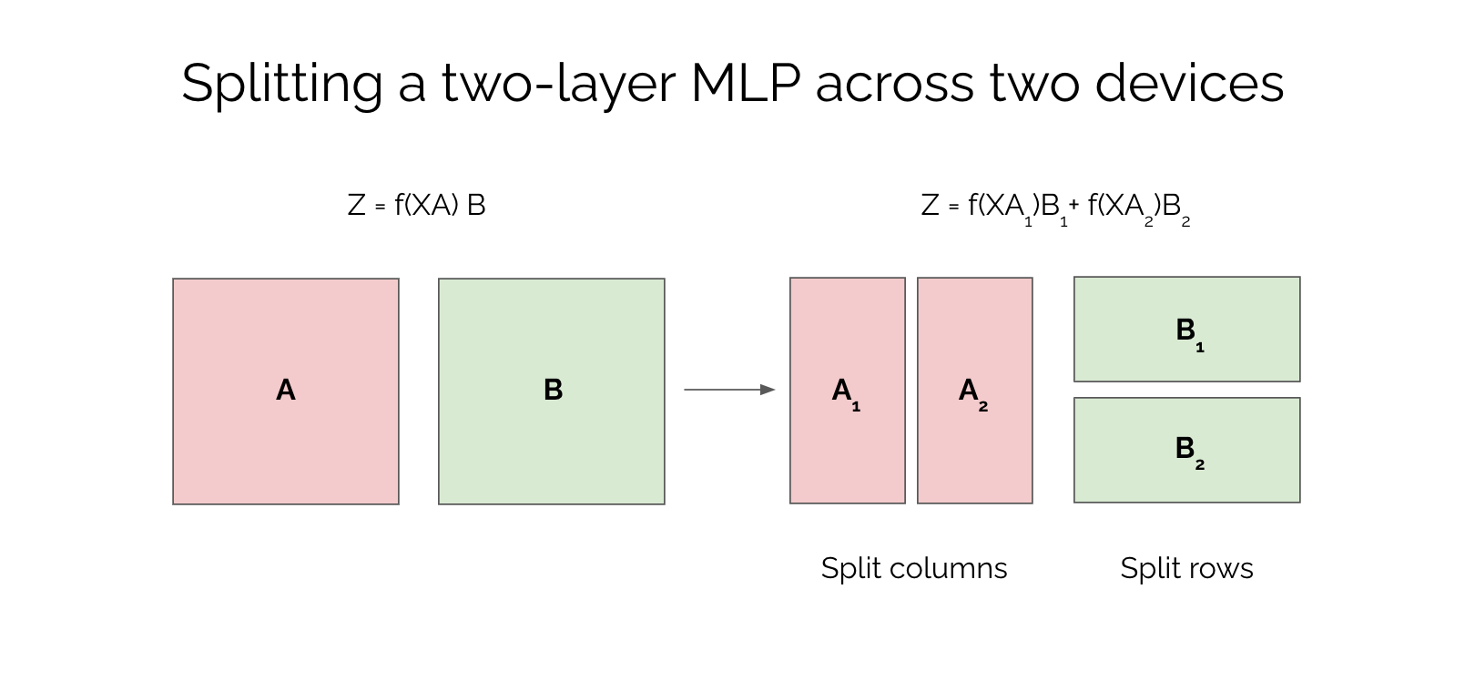
We can split matrix A into two equal parts column-wise, and matrix B into two equal parts row-wise. We can represent matrix A as , and matrix B as . Here, and are the two equal parts of matrix A, and and are the two equal parts of matrix B. If we substitute these matrices into the computation, we get:
and where the two computations that were happening on separate devices are joined with an allreduce operation. This relation follows from linear algebra, because so these two computations can be done independently in parallel.
We have just described a tensor parallel forward pass. But what about the backward pass? The backward pass is a bit more complicated, because we need to compute the gradients of the loss with respect to the parameters. In the forward pass, we computed and . So the gradients of the loss with respect to and are:
where and are the gradients of the loss with respect to the output of the first and second layers, respectively. We can compute these gradients with the chain rule. For example, and backpropagate the error from the global loss value computed after the forward pass.
Illustrative example of tensor parallelism with Numpy
To make things more concrete, let's see how we can implement a tensor parallel MLP in Numpy. We'll use the same example as before, where we have a 2 layer MLP with layer 1 parameterized by matrix A and layer 2 parameterized by matrix B. We'll use the same notation as before, where and are the two equal parts of matrix A, and and are the two equal parts of matrix B. We'll also use the same activation function as before.
We'll start by defining a function that splits a matrix into two equal parts column-wise. We'll use the numpy.split (opens in a new tab) function to do this. We'll also define a function that splits a matrix into two equal parts row-wise.
import numpy as np

def split_columnwise(A, num_splits):
    return np.split(A, num_splits, axis=1)

def split_rowwise(A, num_splits):
    return np.split(A, num_splits, axis=0)
Now, let's define a function that computes the forward pass of a tensor parallel MLP. We'll use the numpy.dot (opens in a new tab) function to compute the matrix multiplication. We'll also use the numpy.sum (opens in a new tab) function to compute the sum of the two parts of the output.
def normal_forward_pass(X, A, B, f):
  Y = f(np.dot(X, A))
  Z = np.dot(Y, B)
  return Z

def tensor_parallel_forward_pass(X, A, B, f):
    A1, A2 = split_columnwise(A, 2)
    B1, B2 = split_rowwise(B, 2)
    Y1 = f(np.dot(X, A1))
    Y2 = f(np.dot(X, A2))
    Z1 = np.dot(Y1, B1)
    Z2 = np.dot(Y2, B2)
    Z = np.sum([Z1, Z2], axis=0)
    return Z
We can now compute the forward pass of the MLP. We'll use the numpy.random.randn (opens in a new tab) function to generate random matrices.
X = np.random.randn(2, 2)
A = np.random.randn(2, 2)
B = np.random.randn(2, 2)
Z = tensor_parallel_forward_pass(X, A, B, np.tanh)
Z_normal = normal_forward_pass(X, A, B, np.tanh)
print(np.allclose(Z, Z_normal)) # outputs: True
Suppose we are doing regression with this MLP and that the true targets are . We can compute the loss as follows.
target = np.array([[-0.5, 0.5], [-0.5, 0.5]])
# loss function
def L(Z, Y):
    return np.sum((Z - Y) ** 2)
loss = L(Z, target)
Now we can also compute the backward pass of the MLP with respect to this loss. First, let's forget about tensor parallelism and derive the backpropagation equations in code for the normal MLP. Specifically, we want to know how to adjust the weight matrices and to reduce the loss, or in other words, how to compute the gradients of the loss with respect to and .
def normal_backward_pass(X, A, B, f):
    # recompute forward pass to get activations
    Y = f(np.dot(X, A))
    Z = np.dot(Y, B)
    # compute gradients
    # gradient of loss with respect to Z
    dLdZ = 2 * (Z - Y)
    # gradient of loss with respect to B via chain rule
    # dLdB = dLdZ * dZdB = dLdZ * Y = np.dot(Y.T, dLdZ)
    dLdB = np.dot(Y.T, dLdZ)
    # gradient of loss with respect to A via chain rule
    # dLdY = dLdZ * dZdY = dLdZ * B = np.dot(dLdZ, B.T)
    dLdY = np.dot(dLdZ, B.T)
    # dLdA = dLdY * dYdA = dLdY * (1 - Y ** 2) = np.dot(X.T, dLdY * (1 - Y ** 2))
    # (1 - Y ** 2) is the derivative of the activation function f = np.tanh
    # derivative of tanh is 1 - tanh ** 2
    dLdA = np.dot(X.T, dLdY * (1 - Y ** 2))
    return dLdA, dLdB, Z
In the above code, we're using the chain rule to compute the gradients and , where is the loss. Since the output of the second layer is used directly for prediction the gradient is straightforward to compute. The tricky part is the term because it requires differentiating through the activation function . In this case, we're using the activation function, so we can use the fact that to compute the derivative of as .
To see how we arrived at the equation for , let's step through the chain rule mathematically. First, we have that . The term is straightforward to compute, so we'll focus on . Let's express this derivative in terms of the output of the activation function and the input to the activation function . We have that , so . Now, we can substitute for to get . This is the same equation we used in the code above.
def tensor_parallel_backward_pass(X, A, B, f):
    # recompute forward pass to get activations
    A1, A2 = split_columnwise(A, 2)
    B1, B2 = split_rowwise(B, 2)
    Y1 = f(np.dot(X, A1))
    Y2 = f(np.dot(X, A2))
    Z1 = np.dot(Y1, B1)
    Z2 = np.dot(Y2, B2)
    Z = Z1 + Z2

    # compute gradients, same logic as from normal_backward_pass
    # this one has to be done without parallelism
    # since dLdZ1 = dLdZ2 = dLdZ
    dLdZ = 2 * (Z - np.concatenate([Y1, Y2], axis=1))

    dLdZ1 = dLdZ
    dLdZ2 = dLdZ

    dLdB1 = np.dot(Y1.T, dLdZ1)
    dLdB2 = np.dot(Y2.T, dLdZ2)

    dLdY1 = np.dot(dLdZ1, B1.T)
    dLdY2 = np.dot(dLdZ2, B2.T)

    dLdA1 = np.dot(X.T, dLdY1 * (1 - Y1 ** 2))
    dLdA2 = np.dot(X.T, dLdY2 * (1 - Y2 ** 2))

    # to sense check our results
    dLdB = np.concatenate([dLdB1, dLdB2], axis=0)
    dLdA = np.concatenate([dLdA1, dLdA2], axis=1)

    return dLdA, dLdB
If you run the code above, you'll see that the normal and tensor parallel implementation match. From a quick glance at the code, we can spot a few subtle details that need to be carefully throught through. First, note that since the gradients are equal. For this reason, these gradients need to be computed on the same device. After this, we can compute all the gradients for and in parallel. Another detail is that to sense check our results we concatenate and on different axes. This is because was split column-wise while was split row-wise. From this example, we can see that tensor parallelism needs to be implemented carefully. It's very easy to introduce silent bugs, which is why tensor parallelism is generally more difficult to implement than data parallelism.
Note that this implementation in numpy is only illustrative. The computation in the code I showed is still done on a single device, but the tensor parallel implementations show the logic that needs to be implemented in a distributed setting. Modern autodiff software like PyTorch and JAX takes care of the details of distributing your computation across multiple devices, but it's important to know the underlying logic since you often still need to specify which parts of your computation should be done in parallel and on which devices.
Finally, parallelizing tensors is highly device specific. You would parallelize differently on a 8x2 vs a 4x4 device topology for instance. In large scale training, tensor parallelism is often combined with data parallelism. For instance, with an MxN device grid you might parallelize the data across the rows and tensors across the columns.
A tensor parallel MLP in JAX
Let's see how we can implement a tensor parallel MLP in JAX. We'll use the same example as before, where we have a 2 layer MLP with layer 1 parameterized by matrix A and layer 2 parameterized by matrix B. We'll use the same notation as before, where and are the two equal parts of matrix A, and and are the two equal parts of matrix B. We'll also use the same activation function as before.
We'll start by defining a function that splits a matrix into two equal parts column-wise. We'll use the jax.numpy.split (opens in a new tab) function to do this. We'll also define a function that splits a matrix into two equal parts row-wise.
import jax
import jax.numpy as jnp

def split_columnwise(A, num_splits):
    return jnp.split(A, num_splits, axis=1)

def split_rowwise(A, num_splits):
    return jnp.split(A, num_splits, axis=0)
Now, let's define a function that computes the forward pass of a tensor parallel MLP. Our function will input the data X, the split matrices A_i and B_i (e.g. A_1 and B_1) and the non-linearity and use pmap to split the computation across multiple devices. We'll use the jax.lax.pmap (opens in a new tab) function to do this.
Recall how we parallelized data in our previous post.
import jax
import jax.numpy as jnp

def linear_layer(x, w):
  return jnp.dot(x, w)

n = 16
d = 3
devices = 8


xs = jnp.array(np.random.rand(n, d))
ws = jnp.array(np.random.rand(d,))

x_parts = np.stack(jnp.split(xs, devices))
w_parts = jax.tree_map(lambda x: np.stack([x for _ in range(devices)]), ws)

out = jax.pmap(linear_layer)(x_parts, w_parts)
print(out.shape) # (8, 2), out is a matrix of shape (n_devices, n_data // n_devices)
Here, the weights were replicated across devices while data was split and parallelized. Now we want to do the opposite - we want to replicate the data and parallelize the model.
import jax
import jax.numpy as jnp

def split_columnwise(A, num_splits):
  return jnp.split(A, num_splits, axis=1)

def split_rowwise(A, num_splits):
  return jnp.split(A, num_splits, axis=0)

def forward(x, a, b):
  y = jnp.tanh(jnp.dot(x, a))
  z = jnp.dot(y, b)
  return z


A_parts = np.stack(split_columnwise(A, devices))
B_parts = np.stack(split_rowwise(B, devices))
X_parts = jax.tree_map(lambda x: np.stack([x for _ in range(devices)]), X)

out = jax.pmap(forward)(X_parts, A_parts, B_parts)

z = jnp.sum(out, axis=0)
Given the same inputs for X,A,B as in the numpy example, we get the same output. Except this time JAX has parallelized the computation across two devices. We can also check that the gradients are correct.
Cross device communication
In the numpy and jax examples, we parallelized the MLP computation across two devices. However, we only addressed the parallelization logic and did not discuss how data is centralized and distributed across devices. For example, at the end of the forward pass we need to sum the outputs of the two devices , but and live on different devices. How do we perform the summation?
In distributed computing, this can be done with an AllReduce operation which performs a reduction (e.g. summation), then processes and distributes the result to all devices. In JAX, we can use the jax.lax.psum (opens in a new tab) function to perform an AllReduce operation.
To compute the loss, we also need to use an Gather operation for this term concatenate([Y1, Y2]). Finally, to distribute the gradients back to the devices, we need to use an Scatter operation.
Megatron
What we've outlined in this post is a form of tensor parallelism that was introduced in the Megatron paper (opens in a new tab) by NVIDIA. Unlike pipeline parallelism, Megatron tensor parallelism is efficient in the sense that there is minimal idle time on the devices, and for this reason it is commonly used for large scale training of language models.