Training Deep Networks with Data Parallelism in Jax

You,Sun Feb 19 2023•large model engineering

One of the main challenges in training large neural networks, whether they are LLMs or VLMs, is that they are too large to fit on a single GPU. To address this issue, their training can be parallelized across multiple GPUs. This means either parallelizing the data or model to distribute computation across several devices. In this post, we'll cover batch splitting, also known as data parallelism, and show how to use JAX's pmap function to parallelize computations across multiple devices.

Parallelizing a 300M GPT model

Let's start with an illustrative example. Suppose we're training GPT model with has 300M parameters on a machine with 8 Tesla V100 GPUs. How can we parallelize the model across GPUs to get a maximally efficient runtime? Since the model has 300M parameters, storing its parameters takes up 1.2GB of RAM (see here (opens in a new tab)). However, the memory footprint for training a transformer model will be dominated by the activations. Let $T, D$ denote the sequence length and hidden dimensions of the model. Assuming $T \gg D$ , the memory footprint of a transformer is roughly (opens in a new tab):

$M \approx M_{model} \frac{BT^2}{4ND^2}$

where $B$ is that batch size and $N$ is the number of attention heads. Now let's assume $T=1024$ , $N=8$ , $D=128$ , then the formula reduces to:

$M \approx 1.2 \cdot 8 B = 9.6 B$

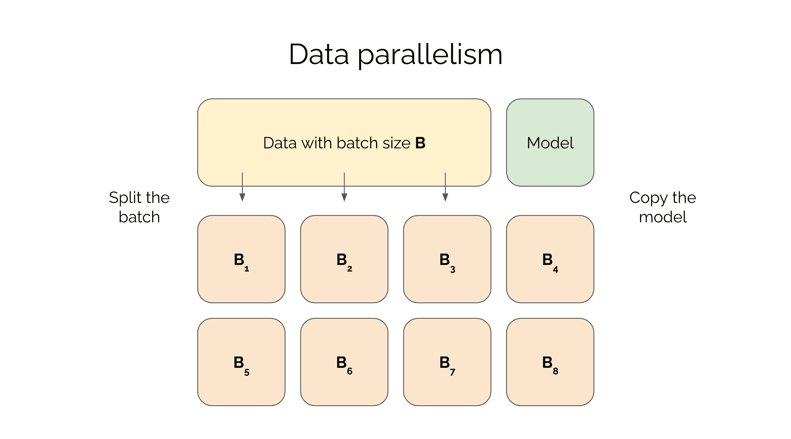
In other words, storing the activations will require around $10$ GB for each batch element when you train your model. Current Tesla V100 GPUs have 32GB of RAM so this means you will be able to fit this model with a batch size of 3 on each device. The optimal training set up is then to have a batch size of $B=24$ and split the the minibatch across 8 devices. Note how you can store the entire model in RAM but the limiting factor is the batch size. This is why this parallelization technique is called data parallelism - you copy the model across each device but parallelize the data.

Data Parallelism in Jax

Let's walk through a simple example of data parallelism in JAX by looking at how to parallelize the forward pass of a linear layer. We'll first show how to pass a single data point through the layer, then multiple points on one device, and finally multiple points across multiple devices.

A linear layer

First, let's define a simple linear layer.

import jax
import jax.numpy as jnp
 
def linear_layer(x, w):
  return jnp.dot(x, w)

One data point

Now let's pass one data point through the linear layer.

d = 3
x = jnp.array(np.random.rand(d))
w = jnp.array(np.random.rand(d))
out = linear_layer(x, w)
print(out.shape) # (), out is a scalar

The output is just a scalar.

Multiple data points on one device

To efficiently pass multiple data points on one device we can use the vmap function to apply a function in parallel without worrying about tensor shapes.

n = 16
d = 3
devices = 8
 
 
xs = jnp.array(np.random.rand(n, d))
ws = jnp.array(np.random.rand(d,))
 
out = jax.vmap(linear_layer, in_axes=[0, None])(xs, ws)
print(out.shape) # (16,), out is a vector

The output is a vector of length 16 that is stored on a single device.

Multiple data points on multiple devices

Parallelizing this operation across multiple devices works. By using pmap we get the same vectorized functionality as vmap but on multiple devices.

x_parts = np.stack(jnp.split(xs, devices))
w_parts = jax.tree_map(lambda x: np.stack([x for _ in range(devices)]), ws)
 
out = jax.pmap(linear_layer)(x_parts, w_parts)
print(out.shape) # (8, 2), out is a matrix of shape (n_devices, n_data // n_devices)

The output is a matrix of shape (8, 2) that is stored on 8 devices. When flattened this matrix is equivalent to the vector of length 16 that we got from vmap. The only awkward part about this example is that we replicated the weights across all devices. We can avoid this step if we use in_axes in the pmap function:

out = jax.pmap(linear_layer, in_axes=(0, None))(x_parts, ws)
print(out.shape) # (8, 2), out is a matrix of shape (n_devices, n_data // n_devices)

Data parallelized linear regression

We can now write out an example of how training with data parallelism works. For each minibatch, each device computes the gradients with respect to the parameters and sends them to a central server. The server averages the gradients and sends the result back to each device. Each device then updates its copy of the parameters using the average gradients. This ensures that each device is training the model using the most up-to-date parameters.

Here's a simple example of data parallel linear regression, which I've modified from this colab (opens in a new tab) where you can find a full working example.

from typing import NamedTuple, Tuple
import functools
 
# class for storing model parameters
class Params(NamedTuple):
  weight: jnp.ndarray
  bias: jnp.ndarray
 
# function for initializing model parameters
def init(rng) -> Params:
  """Returns the initial model params."""
  weights_key, bias_key = jax.random.split(rng)
  weight = jax.random.normal(weights_key, ())
  bias = jax.random.normal(bias_key, ())
  return Params(weight, bias)
 
# function for computing the MSE loss
def loss_fn(params: Params, xs: jnp.ndarray, ys: jnp.ndarray) -> jnp.ndarray:
  """Computes the least squares error of the model's predictions on x against y."""
  pred = params.weight * xs + params.bias
  return jnp.mean((pred - ys) ** 2)
 
# function for performing one SGD update step (fwd & bwd pass)
@functools.partial(jax.pmap, axis_name='num_devices')
def update(params: Params, xs: jnp.ndarray, ys: jnp.ndarray) -> Tuple[Params, jnp.ndarray]:
  loss, grads = jax.value_and_grad(loss_fn)(params, xs, ys)
  grads = jax.lax.pmean(grads, axis_name='num_devices')
  loss = jax.lax.pmean(loss, axis_name='num_devices')
  new_params = jax.tree_map(
      lambda param, g: param - g * LEARNING_RATE, params, grads)
 
  return new_params, loss

Here, the functools.partial decorator wraps the update function with a pmap with axis_name='num_devices' as an input argument to pmap. This means that the update function will be applied in parallel across all devices. The pmean function is used to average the gradients across all devices. The pmean function is similar to np.mean but it also takes an axis_name argument. This argument is used to specify which axis to average across. In this case, we average across the num_devices axis but this name is just a placeholder, we can change it to any string (e.g. 'i' or 'data' and it will work the same).

What `pmap` does under the hood

The pmap operation is pretty magical, it automatically parallelizes your data for you. Under the hood, jax.pmap uses XLA (opens in a new tab) (Accelerated Linear Algebra), a domain-specific compiler for linear algebra operations that JAX is built on. XLA compiles our computation into a series of low-level machine instructions that can be executed efficiently on the underlying hardware.

To implement data parallelism using XLA, jax.pmap generates a series of XLA computations that run on each device simultaneously. These computations are then coordinated using a communication protocol to ensure that each device has the correct data to perform its computation and that the results are combined correctly. The protocol that jax.pmap uses to combine the outputs across all devices into a single variable at the end of the computation is called All-Reduce.

All-Reduce is a common communication protocol in distributed computing that allows multiple devices to exchange information and compute an aggregate value. In the case of jax.pmap, the All-Reduce protocol is used to combine the outputs from each device into a single output.

The All-Reduce protocol works by first computing a local sum on each device, then exchanging the partial sums among all devices, and finally computing the global sum of all partial sums. This approach ensures that all devices have access to the most up-to-date information when computing the aggregate value.

Specifically, in the case of jax.pmap, after each device has computed its local result, it sends its result to a central server, which then applies the All-Reduce protocol to compute the aggregate value. The result is then broadcast back to each device, which can then update its local copy of the result.